Decoder Accuracy Improves with Input Rate
Direct-simulation decoder calibration of the input-rate range for later variable-rate PING training.
Abstract
We asked which input rates preserve enough information in filtered MNIST pixel events for nonlinear decoding. We trained 3 decoders on finite-window, nonspiking membrane features and evaluated held-out digits. Mean accuracy increased from 28.6% at 0.1 Hz to 96.1% at 25 Hz. The tested range calibrates this representation and decoder; it does not establish PING-network accuracy or predict performance between tested rates.
Results
Mixed-rate validation trajectories
The retained calibration contains three independently initialized nonlinear decoders trained on fresh encoding draws sampled across the complete input-rate grid (Fig. 1).

Each curve shows validation accuracy by epoch for one of 3 training replicates. Accuracy is the fraction correct across 5000 validation presentations, with input rate sampled uniformly and a fresh encoding draw used for every presentation and epoch.
If mixed-rate training learned digit structure that survived stochastic filtering, validation accuracy should improve across all three training replicates rather than only one trajectory.
Each replicate reached its maximum late in training. The selected epochs were 50, 25, 44, with validation accuracies 77%, 76.4%, 76.8%.
Notes.
- The first occurrence of the maximum validation accuracy selected the checkpoint for each training replicate; later ties did not replace it.
Filtered digit features
A reused illustration shows one MNIST digit after the same finite-window synaptic and membrane filtering at three input rates (Fig. 2).

(A) Reused illustrative input digit and its originally simulated features at (B–D) 0.5, 5 and 25 Hz, respectively. Simulations used 1.2 μS conductance increments, 200 ms presentations and independent encoding draws; feature panels share a 0–65 mV scale.
Because sparse Bernoulli input produces a small, random number of events, reducing the rate should remove responses from different pixels rather than attenuate the whole digit uniformly.
At 0.5 Hz only isolated fragments remained. The digit became progressively more complete at 5 and 25 Hz, consistent with stochastic event loss rather than uniform contrast scaling.
Held-out rate-accuracy curve
The three selected decoders received identical held-out feature vectors and encoding draws. The practical floor required every decoder to reach 50% accuracy at a tested rate (Fig. 3).

Points show mean accuracy across 3 training replicates at each maximum-pixel encoding rate; every replicate received the same 5000 held-out images and encoding draws. Shading spans the minimum–maximum replicate accuracy, not a confidence interval. Rules mark 10% chance and the 50% criterion.
If higher input rates preserved more digit structure, held-out accuracy should rise before approaching a plateau.
Mean accuracy across training replicates increased monotonically from 28.6% at 0.1 Hz to 96.1% at 25 Hz.
The selected floor was 0.5 Hz: all three decoders first crossed the criterion there, and mean accuracy was 63.3%.
The resulting interval is a decoder-relative calibration without interpolation; it does not establish PING-network performance.
Methods
-
Retained computation. We reused a completed calibration containing three trained decoders, their validation histories and their held-out correctness records. We did not rerun feature simulation or decoder training for this article.
-
MNIST partitions. Of the 60000 official training images, the first 20000 trained the decoders and the next 5000 selected checkpoints; the remaining 35000 were unused. Evaluation used the first 5000 images from the separate official test partition, with no overlap.
-
Generate input events. Each normalized pixel intensity generated an independent binary event at integration timestep 0.1 ms:
Here indexes pixels, is the simulation-step index, is event probability, and is maximum-pixel encoding rate in spikes/s; 1000 converts milliseconds to seconds.
-
Filter synaptic conductance. Excitatory conductance , in μS, decayed each step by before an event added . The AMPA time constant was ms and event strength was 1.2 μS.
-
Integrate membrane voltage. During simulation step , the updated conductance was held fixed while each non-spiking membrane voltage obeyed
Capacitance was nF, leak conductance μS, leak reversal mV and excitatory reversal mV. Starting at zero conductance and , voltage advanced by the exact exponential solution for that step. Simulation and decoder arithmetic used single precision.
-
Form pixel features. The feature , in mV, averaged post-update voltages above rest:
Here 200 ms, is the timestep count, and physical time at step is . Fresh encoding draws retained finite-window shot-noise effects without a stationary Gaussian approximation[1].
-
Train mixed-rate decoders. At every epoch, we sampled the input rate for each training and validation presentation uniformly from 0.1, 0.25, 0.5, 1, 2, 5, 10, 25 Hz and generated a fresh encoding draw. Each 784–1024–10 ReLU decoder was trained for 50 epochs using cross-entropy, Adam with learning rate 0.001, no weight decay and batch size 1.
-
Independent training replicates. Stochastic-stream identifiers 42, 43, 44 defined independent model initializations, rate assignments and encoding draws.
-
Select checkpoints. At each of the 50 eligible epochs, validation accuracy was the fraction correct across 5000 validation presentations. The earliest epoch attaining the maximum validation accuracy supplied the selected checkpoint for each training replicate.
-
Evaluate shared test features. Every held-out image was simulated once at each tested rate, and all selected decoders received the same feature vector for that image and rate; the feed-forward decoder had no state across presentations. The predicted class was the class with the largest output logit , and accuracy was measured per training replicate and rate.
-
Aggregate held-out accuracy. For each rate and training replicate, we averaged correctness across 5000 held-out images. We then recorded the mean, minimum and maximum accuracy across the 3 training replicates at each rate.
-
Select the tested interval. The practical floor was the lowest tested rate where every decoder reached 50% accuracy, and the ceiling was the highest tested rate. No interpolation was used; an empty qualifying set was reported as right-censored.
-
Present retained evidence. We redrew the validation trajectories and rate-accuracy summary from recorded measurements, using the aggregation defined above without interpolation. We reused the original finite-window feature illustration unchanged rather than implying a new simulation.
Appendix: Finite-window filtering and interpretation
The Bernoulli input events form shot noise: each produces a discrete conductance jump followed by exponential AMPA decay. These pulses change both the voltage toward which the membrane moves and how quickly it moves there. An event’s effect therefore depends on the voltage and conductance left by earlier events, rather than adding a fixed voltage increment.
At low input rates, a finite presentation may contain no events, one event, or a few arriving at different times. Response statistics can change during the presentation (nonstationary), and their distribution can be asymmetric or concentrated around a few outcomes (non-Gaussian)[1]. Direct simulation retained these count and timing effects rather than replacing them with a steady, bell-shaped approximation.
Neural decoding measures information accessible to a specified readout, not absolute information content or the mechanism by which a biological population uses it[2]. The criterion therefore selects a practical interval for this representation and decoder. Transfer to a PING network requires a separate evaluation; decoding accuracy here does not establish gamma timing benefits.
Network diagrams
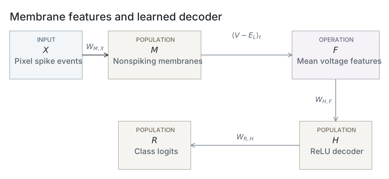
Parameters
This experiment uses an independent nonspiking membrane model. SNNLab spiking-network snapshots do not apply; the schematic above illustrates the independent model. The table reads the selected computation’s recorded configuration; absent evidence stays unavailable.
| Parameter | Recorded value |
|---|---|
| Nonspiking membrane | |
| Capacitance (nF) | 1 |
| Leak conductance (µS) | 0.05 |
| Leak reversal (mV) | -65 |
| Excitatory reversal (mV) | 0 |
| AMPA decay (ms) | 2 |
| Input and simulation | |
| Timestep (ms) | 0.1 |
| Presentation (ms) | 200 |
| Single event strength (µS) | 1.2 |
| Input rates (Hz) | 0.1 / 0.25 / 0.5 / 1 / 2 / 5 / 10 / 25 |
| Numerical precision | float32 |
| Readout and training | |
| Hidden decoder units | 1024 |
| Training images | 20000 |
| Validation images | 5000 |
| Test images | 5000 |
| Epochs | 50 |
| Seeds | 42 / 43 / 44 |
| Checkpoint selection | first_maximum_mixed_rate_validation_accuracy |
Dataset
Upstream: —
Downstream: —
Current runset
| Run | Date | Duration | Size | Evidence | Storage | Ran on | Verification |
|---|---|---|---|---|---|---|---|
| exp080-r003-present | 1s | 123.2 KB | Current | R2 | Local | Local: absent; R2: catalog-verified | |
| exp080-r002-analyse | <1s | 26.4 KB | Current | R2 | Local | Local: absent; R2: catalog-verified | |
| exp080-r001-compute | 1h 36m 51s | 58 KB | Current | R2 | Unknown | Local: absent; R2: catalog-verified |
References
-
Brigham & Destexhe: Nonstationary Filtered Shot-Noise Processes and Applications to Neuronal Membranes. Physical Review E, 2015. doi:10.1103/PhysRevE.91.062102
-
Quian Quiroga & Panzeri: Extracting Information from Neuronal Populations: Information Theory and Decoding Approaches. Nature Reviews Neuroscience, 2009. doi:10.1038/nrn2578