Introduction to Capacitors
Electrons separate onto two plates, creating a voltage and storing energy in an electric field.
Abstract
A capacitor separates electric charge onto two plates. We follow electrons as it charges, holds its charge and discharges, connecting their redistribution to voltage and current. The circuit animation uses schematic electron dots. We then follow a presynaptic spike as it opens a synapse and triggers a neuron's ionic response.
Introduction
A capacitor has two metal plates separated by an insulator. Charging removes electrons from one plate and adds them to the other. The plates acquire equal and opposite net charges; electrons travel through the external wires, never across the insulating gap in this ideal model.[1]
Capacitance , measured in farads (F), relates the upper plate’s positive charge , in coulombs (C), to the voltage difference , in volts (V):
A battery at voltage charges the capacitor through resistance , measured in ohms (Ω). Conventional current , in amperes (A), changes the voltage over time , in seconds (s):[2]
Charging slows as approaches . Hold disconnects the external path; Discharge joins the plates through the resistor. Electron drift runs opposite to conventional current. The time constant , in seconds, sets the charging and discharging timescale:
Choose a mode below, or adjust capacitance, resistance and battery voltage. Blue dots represent electrons. The dots exaggerate size and motion and represent groups of electrons. Changing a slider starts a fresh charge; switching modes preserves voltage. Restart returns to an uncharged capacitor. Pause freezes time. The model omits leakage and dielectric breakdown.
Loading capacitor…
A biophysical neuron
A neuron’s membrane separates conducting fluids and acts as a capacitor. Here the moving charges are ions: sodium () entering the cell can raise its voltage, while potassium () leaving can lower it. Voltage-dependent channels control these flows. The animation uses the classic Hodgkin–Huxley squid-axon membrane model.[3] To receive presynaptic spikes, we add an excitatory synapse; this addition supplies the input current in the voltage equation below.
The membrane voltage is the inside voltage relative to outside, in millivolts (mV). Membrane capacitance per area is in μF/cm²; inward synaptic current density and ionic current densities , and leak are in μA/cm². Time is in milliseconds (ms):
For each pathway , conductance density is in mS/cm² and reversal potential is in mV:
These ionic currents are positive outwards; the current plot reverses their signs so upward means positive charge entering. The reversal potentials are mV, mV and mV. Sodium activation , sodium availability and potassium activation are dimensionless gates between zero and one:
The available maximum conductance densities are and mS/cm². The channel sliders set the fractions and from zero to one, both initially one. Leak conductance is fixed at mS/cm². Each gate evolves as:
The rates and , in ms⁻¹, drive the gate towards one and zero, respectively. With the dimensionless numerical voltage, the animation uses the classical squid-axon rates at 6.3 °C in the inside-minus-outside voltage convention:[3, 4]
Here is the base of the natural exponential. The apparent divisions by zero have finite limits: ms⁻¹ at −40 mV and ms⁻¹ at −55 mV. Each fresh demonstration starts at −65 mV with , then runs for 200 ms without synaptic input before the displayed timeline begins. Membrane capacitance initially equals μF/cm².
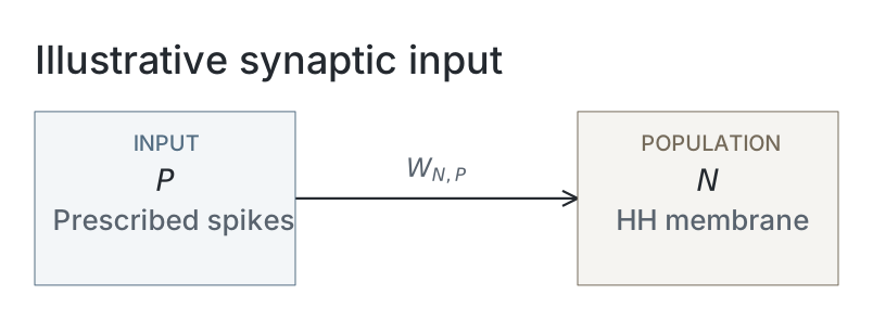
In a biological synapse, an arriving presynaptic spike causes transmitter release, opening synaptic channels. We add a standard conductance-based synapse with instantaneous opening and exponential decay, as described in Neuronal Dynamics, Section 3.1, Equations (3.1)–(3.2). This is an extension to the original Hodgkin–Huxley membrane model.[5] Its conductance density is in mS/cm², and we write its current as inward-positive (the opposite sign convention to that reference):
The synaptic reversal potential is mV. Each arrival adds the selected weight , in mS/cm², to this conductance; between arrivals it decays:
We choose a decay time ms and default weight mS/cm² for this demonstration. The Dirac impulse has unit area and units of ms⁻¹, so each arrival increases conductance by ; this is equivalent to the exponential conductance in the cited model. Arrival times are ms for , following a schematic 4 ms journey from a source with prescribed spikes. These timings are also demonstration choices; transmitter release and the presynaptic neuron’s dynamics are not simulated.
Voltage and the three gates are integrated with fourth-order Runge–Kutta steps of 0.01 ms. Synaptic conductance decays exponentially, evaluated at each step’s start, midpoint and end. Action potentials emerge from the channel dynamics, without a firing threshold or voltage reset. Adjust capacitance, synaptic strength or the available channels to explore the response.
Loading neuron membrane…
Network diagram
Parameters
| Parameter | Illustrative setting |
|---|---|
| Ideal capacitor circuit | |
| Governing relation | Charge equals capacitance times voltage |
| Charge / discharge update | Exact exponential towards battery voltage / zero |
| Hold | Disconnected ideal capacitor; constant voltage |
| Time constant (derived) | Resistance multiplied by capacitance |
| Hodgkin–Huxley membrane | |
| Initial capacitance density | 1 μF/cm² |
| Maximum sodium / potassium conductance densities | 120 / 36 mS/cm² before channel-fraction scaling |
| Leak conductance density | 0.3 mS/cm² |
| Sodium / potassium / leak reversals | 50 / -77 / -54.3 mV |
| Rate convention | Classical squid axon at 6.3 °C; inside-minus-outside voltage |
| Initial voltage / preparation | −65 mV; gates at their voltage-dependent steady state, then 200 ms without input |
| Added synapse and integration | |
| Initial weight / reversal | 0.2 mS/cm² / 0 mV |
| Conductance decay time | 2 ms |
| Prescribed first arrival / subsequent interval | 5 / 40 ms |
| Schematic travel time | 4 ms |
| Integrator / timestep | Fourth-order Runge–Kutta / 0.01 ms |
| Conductance within each step | Exponential values at the start, midpoint and end |
The membrane equations and temperature convention follow the cited classical model; the added synapse, timings and slider settings are demonstration choices. Timing and reversal constants are imported from the animation script. These interactive examples do not depend on a scientific run or saved snapshots.
References
-
Samuel J. Ling, Jeff Sanny and William Moebs. University Physics, Volume 2. OpenStax, 2016. Section 8.1, “Capacitors and Capacitance”. Online section.
-
Samuel J. Ling, Jeff Sanny and William Moebs. University Physics, Volume 2. OpenStax, 2016. Section 10.5, “RC Circuits”. Online section.
-
Alan L. Hodgkin and Andrew F. Huxley. “A quantitative description of membrane current and its application to conduction and excitation in nerve.” The Journal of Physiology 117(4), 500–544, 1952. Paper.
-
NEURON Project. Squid sodium, potassium and leak channel model (hh). Maintained NEURON model implementation, accessed 14 October 2026. Source.
-
Wulfram Gerstner, Werner M. Kistler, Richard Naud and Liam Paninski. Neuronal Dynamics: From Single Neurons to Networks and Models of Cognition. Cambridge University Press, 2014. Chapter 3.1, “Synapses”.