Streaming Control of a Rotary Joint
Joint control with one Elevate neuron per controller, reciprocal inhibition and excitatory sensory feedback in ROS2 Humble.
Abstract
Two single-neuron Elevate controllers drive opposing muscles on a rotary joint with a 2 g tip mass under gravity. Motor spikes activate muscles and inhibit the peer; angle feedback excites each controller. Three ROS2 Humble nodes exchange 1 ms spike windows in Docker on separate CPUs.
Results
Control Approach
The parameters were selected empirically by varying background excitation, sensory feedback strength and muscle response per spike. They remain fixed throughout the displayed recording.
Timings Summary
| Quantity | Value | Meaning |
|---|---|---|
| Internal integration step | 0.025 ms | Integrates neuron equations and detects upward voltage crossings. |
| External simulation step | 1 ms model time | 40 internal steps; fixed input conductances. |
| Exported spike flag | 0 or 1 per neuron per 1 ms | Any upward crossing sets the flag; multiple crossings collapse to one. Finer spike times are discarded. |
| Mechanical step | 1 ms model time | Updates muscle activation, velocity and angle. |
| Model window | 1 ms model time | Model time advanced per callback. |
| Callback | One node update | Advances the model, publishes outputs and records diagnostics. |
| Callback duration | Variable wall time | Execution time, excluding input waiting. |
| Control period | 1 ms wall time | Interval between scheduled releases. |
| Deadline | Scheduled release + 1 ms | Required finish time, even after a late start. |
| Logical transport delay | 1 ms model time | Window 's spikes enter window . |
Mean callback duration (95th percentile): flexor/extensor 0.534 ms (0.702 ms); joint 0.046 ms (0.073 ms).
Of 30,000 callbacks per node, deadline misses were 2,154 flexor (7.18%), 2,183 extensor (7.28%) and 1,480 joint (4.93%). Callbacks over 1 ms: 195 flexor, 218 extensor, 0 joint. Short callbacks can miss deadlines through late starts.
Neuron model
Elevate is a phenomenological model with sodium, potassium, calcium, slow potassium and leak currents:
denote voltage, time, capacitance and applied current. Excitatory and inhibitory conductances have reversals ; intrinsic conductance has reversal . Units are mV, ms, nF, µS and nA; no cell-area calibration is assumed.
For gates ,
is filtered voltage (mV), its timescale (ms), a dimensionless gate, the slope (mV), the midpoint (mV), and the dimensionless sigmoid argument. In that order, slopes are and midpoints mV:
is maximum conductance. Both potassium currents use . KCa depends on filtered voltage, with no calcium-concentration state. All six states, and the five , start at mV.
Numerical update and spike output
Each 1 ms step uses 40 split substeps of ms with fixed input conductances. First update the filters using the old voltage:
The superscript denotes an updated value. Evaluate gates and conductances from , then update the membrane with conductances frozen:
is total conductance (µS), the equilibrium voltage (mV), and indexes the five intrinsic currents. Each frozen sub-update is exact; their composition approximates the coupled dynamics. A crossing mV sets the window’s spike flag without resetting state.
Synaptic and local drive
Let denote flexor or extensor, its peer, and the control window. Synapses decay, then receive spike increments:
and are sensory AMPA and peer GABA conductances (µS). and count the preceding window’s sensory and peer motor spikes. With ms, decay times are ms and per-spike weights are µS. Initial conductances and input counts are zero; increments are added in full, without timestep scaling.
Unfiltered local excitation switches from starting to tonic drive:
is model time from startup, ms, µS and µS. At , the membrane inputs are
and are total excitatory and inhibitory conductances. Recorded settings appear in the parameter table.
Joint dynamics model
Two muscles drive a spring-damped joint. Zero points downward; positive angles point right. Only the tip mass contributes gravity:
is angle (rad); dots denote derivatives in seconds. is base inertia (kg m), tip mass (kg), arm length (m), gravity (m/s), spring rest angle (rad), damping (N m s/rad), and stiffness (N m/rad). are flexor/extensor activations; is maximum muscle torque (N m).
At mechanical step , muscle updates as
Here s, is activation decay time (s), the dimensionless spike increment, and the preceding window’s motor spike count per neuron. Updated activations set torque. Semi-implicit Euler updates velocity, then angle; stops at rad clamp angle and zero velocity.
The joint starts at (90°), with zero velocity and activation. Total inertia is kg m; initial gravity torque is N m. Flexor raises the mass against gravity; extensor lowers it.
Before each update, sensory spikes excite flexor for and extensor for . The sensory centre is , threshold rad, and minimum interspike interval 10 ms. Each channel repeats while beyond threshold.
Architecture Pseudocode
1. Overall
ROS2 Humble runs flexor, extensor and plant as separate processes on separate
CPUs. All three receive the same resolved recipe configuration. Each controller
owns an independent SNNLab stream containing one Elevate neuron; the plant integrates joint mechanics without a neural network.
These Python-like blocks omit boilerplate. ROS2 scheduling and message helpers
are schematic; prepare_stream and stream.advance denote SNNLab’s streaming
interface.
from snnlab.sim import prepare_stream
from torch import float64

cfg = recorded_configuration
dt = cfg["dt_ms"] * ms
nodes = launch_ros2_processes("flexor", "extensor", "plant")
wait_for_ros2_discovery_and_controller_warmup(nodes)
arm_shared_start(nodes, future_ros_time())


def prepare_controller():
    bundle = author_network(cfg)
    stream = prepare_stream(
        bundle,
        window_steps=1,
        batch_size=1,
        device="cpu",
        dtype=float64,
        performance=recorded_performance,
    )
    warm_up_then_reset(stream)
    return stream


def windows(node):
    for n in range(total_windows):
        release = node.monotonic_origin + n * dt
        spin_ros2_until(node, release)
        frames = wait_for_ros2_frames(node, index=n - 1)
        enforce_lag_limit(release)
        with measure_callback(node, deadline=release + dt):
            yield n, frames
            publish_ros2_frame(node, n, node.output_events)
Each node consumes both other nodes’ complete preceding windows from
/frames/flexor, /frames/extensor or /frames/plant. The initial inputs are
empty; every completed window is published, including silence. Late nodes catch
up without dropping windows or shifting deadlines. Callback timing includes
model execution, spike publication and diagnostic buffering, but excludes input
waiting. Buffered diagnostics are exported after control finishes.
2. Flexor node
The flexor receives excitatory sensory spikes from the plant and inhibitory motor spikes from the extensor. Its local excitation is 0.5 µS for the first 20 ms, then 0.04 µS. SNNLab retains membrane and synaptic state between steps.
node = create_ros2_node("flexor")
stream = prepare_controller()

for n, frames in windows(node):
    drive = cfg["flexor_initial_us"] if n * dt < 20 * ms else cfg["tonic_us"]
    inputs = snnlab_inputs(
        tonic=drive,
        sensory=count_sensory_spikes(frames["plant"], channel="flexor"),
        peer=count_spikes(frames["extensor"]),
    )
    result = stream.advance(inputs)
    node.output_events = motor_spike_events(result)
    publish_ros2_spikes("/motor/flexor", node.output_events)
    buffer_voltage_and_spikes(node, result)
3. Extensor node
The extensor receives excitatory sensory spikes from the plant and inhibitory motor spikes from the flexor. Its SNNLab stream is separate from the flexor’s. Local excitation starts at 0 µS for 20 ms, then switches to the same 0.04 µS tonic drive.
node = create_ros2_node("extensor")
stream = prepare_controller()

for n, frames in windows(node):
    drive = cfg["extensor_initial_us"] if n * dt < 20 * ms else cfg["tonic_us"]
    inputs = snnlab_inputs(
        tonic=drive,
        sensory=count_sensory_spikes(frames["plant"], channel="extensor"),
        peer=count_spikes(frames["flexor"]),
    )
    result = stream.advance(inputs)
    node.output_events = motor_spike_events(result)
    publish_ros2_spikes("/motor/extensor", node.output_events)
    buffer_voltage_and_spikes(node, result)
4. Plant/Joint node
The plant receives both controllers’ motor windows. Before advancing mechanics, it encodes the current angle as sensory spikes; motor spikes then update muscle activation and joint motion. Sensory output returns through ROS2 and enters the controllers in the next logical window. This node does not execute SNNLab.
node = create_ros2_node("plant")
joint = Joint(cfg["joint"])

for n, frames in windows(node):
    sensory = joint.encode(n * dt / second)
    motor = [count_spikes(frames["flexor"]), count_spikes(frames["extensor"])]
    joint.advance(motor, dt / second)
    node.output_events = sensory_spike_events(sensory)
    publish_ros2_spikes("/sensory/flexor", sensory[0])
    publish_ros2_spikes("/sensory/extensor", sensory[1])
    buffer_angle_velocity_and_activation(node, joint)
Network diagram
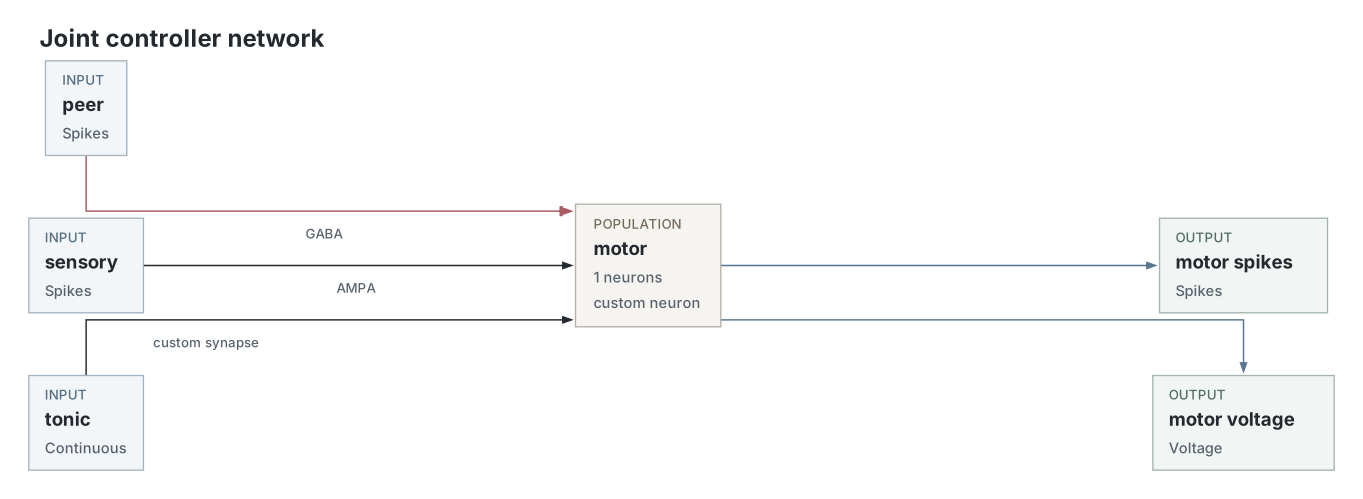
Controller circuit from the saved flexor bundle; both sides use this architecture. is the motor cell, peer spikes, sensory spikes and tonic conductance. Each connection is labelled , with target first and source second. Arrowheads denote excitation; bars denote inhibition. Recording aliases are omitted.
Parameters
Values come from the selected recording’s native snapshot and configuration.
| Parameter | Recorded value |
|---|---|
| Network | |
| Motor cells per controller | 1 |
| Controller populations | motor |
| Neuron model | elevate |
| Ionic membrane dynamics | |
| Capacitance (nF) | 1 |
| Sodium conductance (µS) | 100 |
| Potassium conductance (µS) | 65 |
| Calcium conductance (µS) | 2 |
| Slow potassium conductance (µS) | 10 |
| Leak conductance (µS) | 2 |
| Sodium reversal (mV) | 40 |
| Potassium reversal (mV) | -90 |
| Calcium reversal (mV) | 120 |
| Leak reversal (mV) | -50 |
| Excitation reversal (mV) | 0 |
| Inhibition reversal (mV) | -80 |
| Initial voltage (mV) | -60 |
| Constant applied current (nA) | -5 |
| Sodium activation filter (ms) | 0.1 |
| Sodium inactivation filter (ms) | 1 |
| Potassium activation filter (ms) | 1 |
| Calcium activation filter (ms) | 1 |
| Slow potassium activation filter (ms) | 75 |
| Maximum internal step (ms) | 0.025 |
| Synaptic decay (ms) | |
| local_bias | Direct conductance |
| peer_inhibition | 50 |
| sensory_drive | 10 |
| Synapses and weights | |
| local_bias | 1 |
| peer_inhibition | 0.2 |
| sensory_drive | 0.035 |
| Input and simulation | |
| Duration (s) | 30 |
| Numerical timestep (ms) | 1 |
| Control period (ms) | 1 |
| Seed | 0 |
| Controller warm-up simulated duration (ms) | 1000 |
| Starting pulse duration (ms) | 20 |
| Starting flexor / extensor drive (µS) | 0.5 / 0 |
| Ongoing tonic drive (µS) | 0.04 |
| Spike transport | logical |
| SNNLab execution | default |
| Lag stop / delivery budget (ms) | 8000 / 5 |
| Analysis | |
| Seed count | 1 (selected acquisition) |
| Assessed complete cycles | 10 |
| Cycle burn-in (s) | 5 |
| Cycle relative tolerance | 0.01 |
| Phase samples per cycle | 128 |
| Joint mechanics | |
| Activation increment per normalized spike | 0.003 |
| Activation decay (s) | 0.08 |
| Angle convention | zero_downward_positive_right |
| Arm length (m) | 0.2 |
| Damping (N m s/rad) | 0.02 |
| Gravity (m/s²) | 9.81 |
| Hard stop relative to centre (rad) | 1 |
| Base inertia (kg m²) | 0.005 |
| Initial angle (rad) | 1.5707963267948966 |
| Maximum muscle torque (N m) | 0.8 |
| Sensory and stop centre (rad) | 1.5707963267948966 |
| Minimum sensory interval (s) | 0.01 |
| Sensory threshold relative to centre (rad) | 0.25 |
| Spring rest angle (rad) | 1.5707963267948966 |
| Stiffness (N m/rad) | 0.02 |
| Tip point mass (kg) | 0.002 |
| Total inertia including tip mass (kg m²) | 0.00508 |
Dataset
Upstream: —
Downstream: —
Current runset
| Run | Date | Duration | Size | Evidence | Storage | Ran on | Verification |
|---|---|---|---|---|---|---|---|
| exp152-r116-present | 1s | 19.4 MB | Current | Both | Local | Local: byte-verified; R2: catalog-verified | |
| exp152-r115-analyse | <1s | 4.8 MB | Current | Both | Local | Local: byte-verified; R2: catalog-verified | |
| exp152-r114-compute | 41s | 68.4 MB | Current | Both | Local | Local: byte-verified; R2: catalog-verified | |
| exp152-r113-analyse | <1s | 127.9 KB | Current | Both | Local | Local: byte-verified; R2: catalog-verified | |
| exp152-r112-compute | 36s | 1.9 MB | Current | Both | Local | Local: byte-verified; R2: catalog-verified |
Other stored runs (12)
These runs are outside this experiment's current runset. Their evidence status explains why they remain stored.
| Run | Date | Duration | Size | Evidence | Storage | Ran on | Verification |
|---|---|---|---|---|---|---|---|
| exp152-r155-present | <1s | 13 MB | Unused | R2 | Local | Local: absent; R2: catalog-verified | |
| exp152-r154-analyse | <1s | 2 MB | Unused | R2 | Local | Local: absent; R2: catalog-verified | |
| exp152-r153-compute | 41s | 57.4 MB | Unused | R2 | Local | Local: absent; R2: catalog-verified | |
| exp152-r152-present | <1s | 3.5 MB | Unused | R2 | Local | Local: absent; R2: catalog-verified | |
| exp152-r151-analyse | <1s | 692.5 KB | Unused | R2 | Local | Local: absent; R2: catalog-verified | |
| exp152-r150-compute | 19s | 15.4 MB | Unused | R2 | Local | Local: absent; R2: catalog-verified | |
| exp152-r149-present | 1s | 5.1 MB | Unused | R2 | Local | Local: absent; R2: catalog-verified | |
| exp152-r148-present | 1s | 20.4 MB | Unused | R2 | Local | Local: absent; R2: catalog-verified | |
| exp152-r147-analyse | <1s | 3 MB | Unused | R2 | Local | Local: absent; R2: catalog-verified | |
| exp152-r146-compute | 45s | 2.6 MB | Unused | R2 | Local | Local: absent; R2: catalog-verified | |
| exp152-r136-analyse | <1s | 1.6 MB | Unused | R2 | Local | Local: absent; R2: catalog-verified | |
| exp152-r135-compute | 22s | 18.1 MB | Unused | R2 | Local | Local: absent; R2: catalog-verified |