Mean-field Coupling

A matched phase-locking map and E/I coupling-onset display for delayed mean-field circuits with a self-contained neuronal reference.

Experiment

exp153

Created

25 Oct 26

Updated

29 Oct 26

Collections

Experiments
CTC Attention

Abstract

We measured finite-time phase locking in two locally defined delayed mean-field circuits. Across 143 conditions, 143 passed rhythm and uncoupled-calibration checks and 51 met locking criteria. Both figures use the same map run. Parameters were selected for qualitative agreement with exp133’s onset and coupling displays. These exploratory measurements describe one seeded reference and constant initial history; the closure omits finite-population fluctuations.

Results

Reciprocal coupling and phase locking

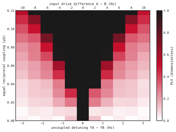
Mean-field PLV across reciprocal coupling and measured uncoupled frequency detuning, with input difference above. — **Figure 1.**
Each rectangle is one sampled setting. Bottom: uncoupled A-minus-B frequency difference (Hz); top: A-minus-B input difference (Hz per channel). Vertical axis: equal nominal total coupling per pathway (µS). White–red–black indicates increasing PLV; gray marks invalid rhythms or an invalid uncoupled calibration. Values use common phase-valid samples within 800–5,000 ms. Cell edges delimit sampled settings. If detuning is unavailable or duplicated, columns retain input spacing and the lower axis explicitly identifies that convention. Nearly matched uncoupled deterministic rhythms can also have high PLV over this finite window; high PLV alone does not establish a coupling effect. Figure 1 uses the locally initialized 14-pathway circuit.

Switching on reciprocal coupling

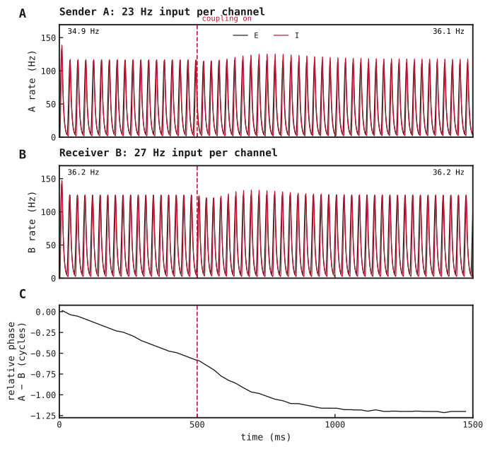
Sender A and receiver B excitatory and inhibitory rates over 1,500 ms, with coupling starting at 500 ms and unwrapped relative phase beneath. — **Figure 2.**
(A) Sender A and (B) receiver B population rates in Hz: excitatory in black, inhibitory in red, with shared rate limits. Input rates are 23/27 Hz per channel for A/B at the selected -4 Hz difference. Dashed lines mark coupling onset at 500 ms. Corner values give E-rhythm frequency over 0–500 ms and 1,000–1,500 ms; a dash indicates an invalid rhythm estimate. (C) Unwrapped A-minus-B E-rate phase in cycles, interpolated only between observed peaks. Phase starts at zero at each circuit’s first detected peak and is never reset at coupling onset. Phase statistics use shared valid times within 800–1,500 ms; unavailable phase is labelled explicitly. Peak times use the 0.5 ms observation grid, which limits phase precision.

Methods

Define. The standalone recipe initializes its own fourteen-pathway neuronal reference and reduces incoming weight sums and explicit delays to four population rates and fourteen conductance filters. Gain settings are recorded with each native model. Local recurrence and rate relaxation were selected to produce sustained oscillatory rates; cross-circuit timing was explored while checking both the onset display and coupling map. This is qualitative parameter selection, not an independent validation against exp133.
Integrate. Use DOP853 with constant prehistory, initial rates of 1 Hz and zero conductances. Table A1 gives the grid, timing and numerical settings; the native exports retain the complete configuration.
Measure. For a full map, derive phase from E-rate peaks and calculate PLV, drift and span, requiring sustained rhythms and valid uncoupled calibration. Extract the onset display from the selected map trajectory, or from a separately recorded onset-only calculation when only Figure 2 is refreshed.

The equations below describe the saved model used for Figure 2; historical equations retain their original architecture. The closure omits input covariance, finite-population fluctuations, weight heterogeneity, voltage-dependent driving forces and shunting; it is not a delayed stability proof.

Circuits are superscripts A/B; E/I denote excitatory/inhibitory populations. For a pathway such as AE → BI, the first pair identifies its source and the second its target; xA/xB denote private sensory inputs. Attention inputs are omitted from the current reduction. All 18 dynamical equations and their current definitions are shown below.

Population-rate functions

\begin{aligned}\tau_{r,E}^{A}\,\dot{r_{E}^{A}} &= - r_{E}^{A} + \Phi_{E}^{A}{\left(I_{E}^{A} \right)} \\ \tau_{r,I}^{A}\,\dot{r_{I}^{A}} &= - r_{I}^{A} + \Phi_{I}^{A}{\left(I_{I}^{A} \right)} \\ \tau_{r,E}^{B}\,\dot{r_{E}^{B}} &= - r_{E}^{B} + \Phi_{E}^{B}{\left(I_{E}^{B} \right)} \\ \tau_{r,I}^{B}\,\dot{r_{I}^{B}} &= - r_{I}^{B} + \Phi_{I}^{B}{\left(I_{I}^{B} \right)}\end{aligned}

Conductance-filter functions

\begin{aligned}\dot{g_{AE\to AE}} &= - \frac{g_{AE\to AE}}{\tau_{AE\to AE}} + \frac{C_{AE\to AE} r_{E}^{A}(t-0.1) a_{AE\to AE}}{1000} \\ \dot{g_{AE\to AI}} &= - \frac{g_{AE\to AI}}{\tau_{AE\to AI}} + \frac{C_{AE\to AI} r_{E}^{A}(t-0.1) a_{AE\to AI}}{1000} \\ \dot{g_{AE\to BE}} &= - \frac{g_{AE\to BE}}{\tau_{AE\to BE}} + \frac{C_{AE\to BE} r_{E}^{A}(t-2) a_{AE\to BE}}{1000} \\ \dot{g_{AE\to BI}} &= - \frac{g_{AE\to BI}}{\tau_{AE\to BI}} + \frac{C_{AE\to BI} r_{E}^{A}(t-2) a_{AE\to BI}}{1000} \\ \dot{g_{AI\to AE}} &= - \frac{g_{AI\to AE}}{\tau_{AI\to AE}} + \frac{C_{AI\to AE} r_{I}^{A}(t-0.1) a_{AI\to AE}}{1000} \\ \dot{g_{AI\to AI}} &= - \frac{g_{AI\to AI}}{\tau_{AI\to AI}} + \frac{C_{AI\to AI} r_{I}^{A}(t-0.1) a_{AI\to AI}}{1000} \\ \dot{g_{xA\to AE}} &= - \frac{g_{xA\to AE}}{\tau_{xA\to AE}} + \frac{C_{xA\to AE} a_{xA\to AE} \nu^{A}}{1000} \\ \dot{g_{BE\to BE}} &= - \frac{g_{BE\to BE}}{\tau_{BE\to BE}} + \frac{C_{BE\to BE} r_{E}^{B}(t-0.1) a_{BE\to BE}}{1000} \\ \dot{g_{BE\to BI}} &= - \frac{g_{BE\to BI}}{\tau_{BE\to BI}} + \frac{C_{BE\to BI} r_{E}^{B}(t-0.1) a_{BE\to BI}}{1000} \\ \dot{g_{BE\to AE}} &= - \frac{g_{BE\to AE}}{\tau_{BE\to AE}} + \frac{C_{BE\to AE} r_{E}^{B}(t-2) a_{BE\to AE}}{1000} \\ \dot{g_{BE\to AI}} &= - \frac{g_{BE\to AI}}{\tau_{BE\to AI}} + \frac{C_{BE\to AI} r_{E}^{B}(t-2) a_{BE\to AI}}{1000} \\ \dot{g_{BI\to BE}} &= - \frac{g_{BI\to BE}}{\tau_{BI\to BE}} + \frac{C_{BI\to BE} r_{I}^{B}(t-0.1) a_{BI\to BE}}{1000} \\ \dot{g_{BI\to BI}} &= - \frac{g_{BI\to BI}}{\tau_{BI\to BI}} + \frac{C_{BI\to BI} r_{I}^{B}(t-0.1) a_{BI\to BI}}{1000} \\ \dot{g_{xB\to BE}} &= - \frac{g_{xB\to BE}}{\tau_{xB\to BE}} + \frac{C_{xB\to BE} a_{xB\to BE} \nu^{B}}{1000}\end{aligned}

Effective currents

\begin{aligned}I_{E}^{A} &= I_{\mathrm{ext},E}^{A} + \Delta V_{e,E}^{A} \left(g_{AE\to AE} + g_{xA\to AE} + g_{BE\to AE}\right) - \Delta V_{i,E}^{A} g_{AI\to AE} \\ I_{I}^{A} &= I_{\mathrm{ext},I}^{A} + \Delta V_{e,I}^{A} \left(g_{AE\to AI} + g_{BE\to AI}\right) - \Delta V_{i,I}^{A} g_{AI\to AI} \\ I_{E}^{B} &= I_{\mathrm{ext},E}^{B} + \Delta V_{e,E}^{B} \left(g_{AE\to BE} + g_{BE\to BE} + g_{xB\to BE}\right) - \Delta V_{i,E}^{B} g_{BI\to BE} \\ I_{I}^{B} &= I_{\mathrm{ext},I}^{B} + \Delta V_{e,I}^{B} \left(g_{AE\to BI} + g_{BE\to BI}\right) - \Delta V_{i,I}^{B} g_{BI\to BI}\end{aligned}

Time is in ms; dots denote time derivatives. Symbols: r, rate (Hz);g, conductance (µS); I, current (nA); τ, relaxation or decay time (ms); C, mean incoming weight (µS); a, dimensionless delivery-time gain; ΔV, fixed driving force (mV); Φ, noisy-LIF current-to-rate function; ν, external input rate (Hz). Subscript ext denotes applied current; e/i denote excitatory/inhibitory driving forces. Cross-circuit gains switch from zero to one at 500 ms; other gains are constant. The factor 1/1000 converts Hz to events per ms.

Network

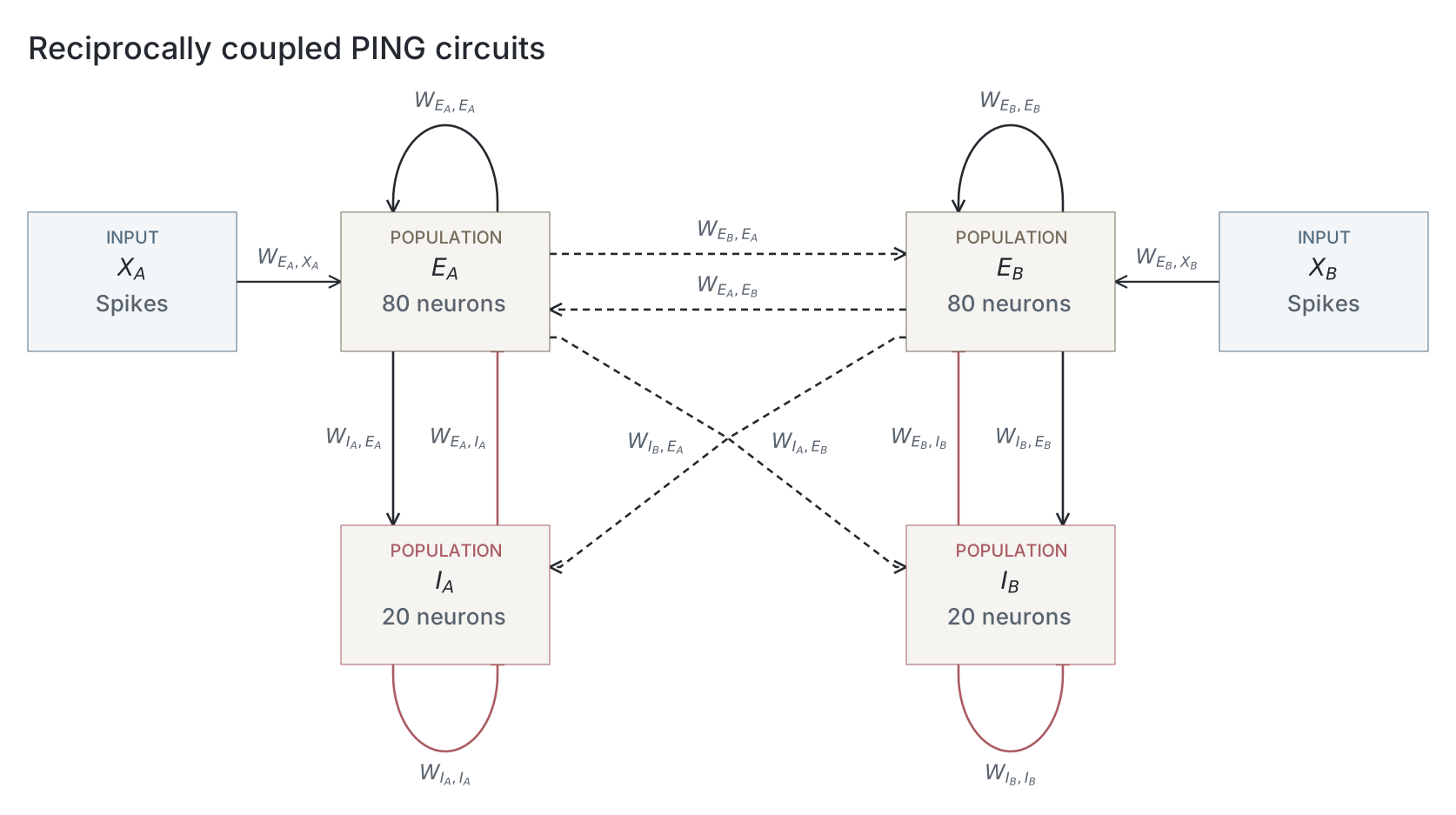
Saved paired PING circuits, with reciprocal excitation from each E population to the other circuit's E and I populations. — **Figure A1.**
Circuit diagram generated from the saved native bundle used in the reduction. Two 80-E/20-I circuits retain their separate external source pools. The mean-field model replaces each population by one rate and each incoming pathway by a conductance filter; neuron counts define incoming weight sums, rather than the number of dynamical rate variables. $E_A$ , $I_A$ , $E_B$ and $I_B$ identify the circuit populations; $X_A$ and $X_B$ are their input pools. Every connection is labelled $W_{XY}$ , with target $X$ first and source $Y$ second. Dashed paths connect circuits; solid paths are local. Arrowheads denote excitation; bars denote inhibition. For the revised circuit, both circuits include local E→E and I→I recurrence without self-connections. Attention inputs are omitted from the current reduction. Node positions, self-loops, routing and weight-label styling align the E/I pairs in columns.

Parameters

The retained native snapshot describes the neuronal reference for the selected presentation. When Figure 1 is preserved from an earlier presentation, it retains that presentation’s original configuration and provenance. The standalone recipe initializes these weights locally without advancing a spiking simulation. Numerical integration settings and closure choices come from the selected exp153 compute record. Reference cross-circuit sums are multiplied by nominal coupling divided by 0.12 µS; the zero-coupling row supplies one uncoupled calibration for each input difference. The current recipe follows exp133’s architecture, with locally selected recurrent strengths, rate relaxation and cross-circuit timing. It applies sensory gain once to the initialized input sums during reduction. Earlier standalone runs embedded that gain in initialization; the selected record determines its application. Connectivity is not resampled.

Parameter	Coupling map	Onset excerpt
Simulation
Integrator / timestep, $dt$	DOP853; adaptive, dt inapplicable	DOP853; adaptive, dt inapplicable
Maximum step / observation interval	0.10 / 0.50 ms	0.10 / 0.50 ms
Analysed duration	5,000 ms	0.0–1,500 ms
Coupling onset	500 ms; continuous state	500 ms; continuous state
Weight-initialization seed	85	85
Populations
$E_A$	80 conductance-LIF reference neurons	80 conductance-LIF reference neurons
$I_A$	20 conductance-LIF reference neurons	20 conductance-LIF reference neurons
$E_B$	80 conductance-LIF reference neurons	80 conductance-LIF reference neurons
$I_B$	20 conductance-LIF reference neurons	20 conductance-LIF reference neurons
$X_A$	1,000 input channels	1,000 input channels
$X_B$	1,000 input channels	1,000 input channels
Neuron dynamics
Rate relaxation, E / I	5.0 / 5.0 ms	5.0 / 5.0 ms
Reference membrane time constant, E / I	20 / 5.0 ms	20 / 5.0 ms
Reference refractory period, E / I	3.0 / 1.5 ms	3.0 / 1.5 ms
Input and manipulation
Private input rate, A / B (Hz/channel)	20 to 30 (step 1.0) / 30 to 20 (step -1.0)	23 / 27
A-minus-B input difference (Hz/channel)	-10 to 10 (step 2.0)	-4.0
Coupling per cross-circuit pathway (µS)	0.0 to 0.12 (step 0.010)	0.090
Measurement
Phase measurement window	800–5,000 ms	800–1,500 ms

Table A1. Recorded mean-field settings and saved neuronal-reference populations for Figures 1 and 2. E / I denotes excitatory / inhibitory; LIF means leaky integrate-and-fire; X identifies private sensory input. Each neuronal population becomes one continuous rate; each retained pathway becomes a conductance filter. The initialization seed identifies the weight draw, not independent repetitions. Sensory rates are deterministic. The onset calculation uses its recorded trajectory. Quantities use two significant figures; seed identifiers remain exact.

Source ↓ / target →	$E_A$	$I_A$	$E_B$	$I_B$
$E_A$	100%; 5.0	100%; 9.4 ± 0.94	10%; 11	10%; 11
$I_A$	100%; 75 ± 7.5	100%; 40	Absent	Absent
$E_B$	10%; 11	10%; 11	100%; 5.0	100%; 9.4 ± 0.94
$I_B$	Absent	Absent	100%; 75 ± 7.5	100%; 40
$X_A$	100%; 1.8 ± 0.27	Absent	Absent	Absent
$X_B$	Absent	Absent	100%; 1.8 ± 0.27	Absent

Table A2. Connectivity of the saved Figure 2 reference, illustrated at -4.0 Hz input difference and 0.090 µS coupling after onset. Rows are sources; columns are targets. Each cell gives eligible-pair density and nominal spiking-reference weight in nS per connection (mean ± SD for random initializers). Weights include saved execution scaling and post-onset gain; they are not measured matrix statistics or total incoming conductances. Self-connections are excluded on the diagonal; cross-circuit paths use exact fan-in. Absent means no retained projection. The reduction uses measured matrix sums divided by target count, with recorded sensory gain and cross-circuit sums scaled to this condition. Synaptic decay / delay: E→E AMPA 2.0 / 0.10 ms; E→I AMPA 1.0 / 0.10 ms; Cross-circuit excitation AMPA 0.50 / 2.0 ms; I→E GABA 9.0 / 0.10 ms; I→I GABA 6.0 / 0.10 ms; Sensory input AMPA 2.0 / 0.0 ms.

The native mean-field model document records symbolic equations and delayed dependencies. Each trajectory retains its constant history, actual parameters, delivery-time controls and solver settings. These finite-time measurements do not constitute a delayed stability proof. See the mean-field note for the stationary-gain closure and its limitations.

Dataset

Upstream: —

Downstream: —

Current runset

Run	Date	Duration	Size	Evidence	Storage	Ran on	Verification
exp153-r045-present	29 Oct 2026, 17:43	12s	1.8 MB	Current	Local	Local	Local: metadata-validated; R2: absent
exp153-r044-analyse	29 Oct 2026, 17:42	7s	714.5 KB	Current	Local	Local	Local: metadata-validated; R2: absent
exp153-r043-compute	29 Oct 2026, 17:08	19m 59s	715.6 MB	Current	Local	Unknown	Local: metadata-validated; R2: absent

Other stored runs (26)

These runs are outside this experiment's current runset. Their evidence status explains why they remain stored.

Run	Date	Duration	Size	Evidence	Storage	Ran on	Verification
exp153-r042-analyse	29 Oct 2026, 17:06	<1s	213.7 KB	Unused	Local	Local	Local: metadata-validated; R2: absent
exp153-r041-analyse	29 Oct 2026, 17:06	<1s	214.1 KB	Unused	Local	Local	Local: metadata-validated; R2: absent
exp153-r040-compute	29 Oct 2026, 17:04	37s	2.2 MB	Unused	Local	Unknown	Local: metadata-validated; R2: absent
exp153-r039-compute	29 Oct 2026, 17:04	37s	2.2 MB	Unused	Local	Unknown	Local: metadata-validated; R2: absent
exp153-r038-analyse	29 Oct 2026, 17:04	1s	214.3 KB	Unused	Local	Local	Local: metadata-validated; R2: absent
exp153-r037-analyse	29 Oct 2026, 17:02	<1s	214.1 KB	Unused	Local	Local	Local: metadata-validated; R2: absent
exp153-r036-compute	29 Oct 2026, 17:01	34s	2.2 MB	Unused	Local	Unknown	Local: metadata-validated; R2: absent
exp153-r035-compute	29 Oct 2026, 17:00	36s	2.2 MB	Unused	Local	Unknown	Local: metadata-validated; R2: absent
exp153-r034-analyse	29 Oct 2026, 16:59	<1s	214.8 KB	Unused	Local	Local	Local: metadata-validated; R2: absent
exp153-r033-compute	29 Oct 2026, 16:57	36s	2.2 MB	Unused	Local	Unknown	Local: metadata-validated; R2: absent
exp153-r032-analyse	29 Oct 2026, 16:56	<1s	215.7 KB	Unused	Local	Local	Local: metadata-validated; R2: absent
exp153-r031-compute	29 Oct 2026, 16:52	3m 45s	2.2 MB	Unused	Local	Local	Local: metadata-validated; R2: absent
exp153-r030-present	29 Oct 2026, 16:51	14s	1.8 MB	Unused	Local	Local	Local: metadata-validated; R2: absent
exp153-r029-analyse	29 Oct 2026, 16:50	6s	716.5 KB	Unused	Local	Local	Local: metadata-validated; R2: absent
exp153-r028-compute	29 Oct 2026, 16:28	10m 19s	712.8 MB	Unused	Local	Unknown	Local: metadata-validated; R2: absent
exp153-r027-analyse	29 Oct 2026, 16:18	<1s	215.9 KB	Unused	Local	Local	Local: metadata-validated; R2: absent
exp153-r026-compute	29 Oct 2026, 16:17	1m 1s	2.2 MB	Unused	Local	Local	Local: metadata-validated; R2: absent
exp153-r025-analyse	29 Oct 2026, 16:16	<1s	45.2 KB	Unused	Local	Local	Local: metadata-validated; R2: absent
exp153-r024-compute	29 Oct 2026, 16:14	1m 10s	2.2 MB	Unused	Local	Local	Local: metadata-validated; R2: absent
exp153-r023-analyse	29 Oct 2026, 16:13	<1s	48.6 KB	Unused	Local	Local	Local: metadata-validated; R2: absent
exp153-r022-compute	29 Oct 2026, 16:12	1m 5s	2.2 MB	Unused	Local	Local	Local: metadata-validated; R2: absent
exp153-r021-analyse	29 Oct 2026, 16:11	<1s	45.3 KB	Unused	Local	Local	Local: metadata-validated; R2: absent
exp153-r020-compute	29 Oct 2026, 16:10	1m 9s	2.2 MB	Unused	Local	Local	Local: metadata-validated; R2: absent
exp153-r019-present	25 Oct 2026, 18:46	<1s	594 KB	Required by deployment:40549382638/1	R2	Local	Local: absent; R2: catalog-verified
exp153-r017-analyse	25 Oct 2026, 18:44	<1s	366.7 KB	Required by deployment:40549382638/1	R2	Local	Local: absent; R2: catalog-verified
exp153-r016-compute	25 Oct 2026, 18:43	15s	4.3 MB	Required by deployment:40549382638/1	R2	Local	Local: absent; R2: catalog-verified