Pinglab Rythmicity Metric
Lobe–trough contrast across untrained PING coupling strengths, with private- and shared-input null controls.
Abstract
We swept an 11×11 reciprocal-coupling grid in an untrained PING circuit and compared autocorrelation contrast with private- and shared-input null controls. At seed 42, selected diagonal conditions had lobe–trough contrasts 0.000301, 0.268 and 0.989. Coupled conditions generally showed stronger temporal structure, but shared input could also produce elevated contrast without feedback. These single-seed observations do not establish rate invariance or the spiking transition’s bifurcation type.
Results
Coupling-map structure
On either zero-coupling edge the loop was broken: E fired at 168.91 Hz and contrast was 0.000301, while I was silent when E-to-I coupling was zero. The diagonal examples in panels D/E/F had contrasts 0.000301/0.268/0.989. Coupled conditions generally showed stronger temporal structure, although the map was not strictly monotonic (Fig. 1).

(A–C) Per-neuron E rate, I rate and lobe–trough contrast, respectively, across the 11×11 coupling grid; and denote E-to-I and I-to-E coupling strengths. The high I rate on one zero edge is colour-clipped. (D–F) Rasters at the diagonal conditions marked D, E and F in panel C, respectively; E spikes are black and I spikes red. Each raster shows 200 ms from the first 160 E and 48 I neurons. One seed per condition; no uncertainty estimate.
Coupled-grid rasters
Many coupled-interior conditions showed separated volleys, whereas the zero-E-to-I column had silent I neurons and the zero-I-to-E row lacked inhibitory feedback to E (Fig. 2).

(A–AJ) E/I rasters at a 6×6 subset of coupling coordinates, ordered row-major from high to low and low to high ; the maps above use all 121 conditions. Display windows and neuron subsets match Figure 1; measurements use all neurons over the full post-burn recording.
Coupled-grid autocorrelograms
Edge autocorrelograms remained near chance. In the coupled interior, short-lag clustering, suppression between volleys and later recurrence peaks supplied complementary temporal evidence (Fig. 3).

(A–AJ) E-population autocorrelograms at the same 6×6 coordinates and in the same row-major coupling order, shown over 0–50 ms. Dotted lines mark the chance reference ; markers locate the selected lobe (▲) and trough (▼) of the smoothed curve. scores the first lobe and trough, not the later peak’s frequency.
Input-sharing controls
Without an inhibitory loop, the private-input null had a maximum contrast of 0.0392 over 2.00–168.91 Hz. The shared-input null reached 1 at 0.0109 Hz, but that estimate contained only 10 E spikes across the population. At 1.39 Hz its contrast was 0.127. Shared afferents can create short-lag coincidence detected by this score; the sparse extreme also illustrates its finite-sample sensitivity. These single-seed controls do not prove rate invariance or establish rhythmicity from contrast alone (Fig. 4).

Contrast against measured E firing rate. Black and grey points are the private- and shared-input nulls; red points are the PING coupling grid, including its near-zero edges.
Rate-matched null structure
Shared-input examples showed central coincidence without inhibitory feedback; private-input examples showed smaller contrast and finite-sample fluctuations around chance. Their approximate rate matching did not make rates or spike counts equal (Fig. 5).

Null autocorrelograms nearest to target E rates of 1, 2.5 and 5 Hz. Shared-input examples (A–C) fired at 1.39/1.39/3.94 Hz; private-input examples (D–F) at 2.00/2.00/3.96 Hz. Within each input type, the first two targets selected the same recording; these are repeated displays, not independent observations.
Methods
-
Sweep coupling. We simulated untrained PING networks (1,024 E/256 I neurons) at 11×11 combinations of –3 µS and –6 µS. Each E neuron received private 100 Hz Poisson input with identity weight 0.5. Settings were: GABA decay 6 ms; E/I reset holds 1.2/0.6 ms; seed 42; one trial; 0.1 ms steps; 1,000 ms duration, discarding the first 100 ms.
-
Test input sharing. With both couplings zero, we scanned private input at 1/2/5/10/20/40/70/100 Hz and shared input at 8/12/16/20/28/40/60/100 Hz. Shared input used 200 channels, weight 0.2 and 95% initial zeros. Reusing the grid’s 100 Hz private origin gave 136 unique probes.
-
Measure rates and autocorrelation. Per-neuron rates were post-burn spike counts divided by population size and 0.9 s. For E counts in bins of width ms, we calculated
Here is normalized autocorrelation, indexes bins, is their mean count, and gives lag . We used zero-padded FFT correlation with overlap and squared-mean normalization: chance reference 1, zero lag excluded.
-
Calculate lobe–trough contrast. After filling zero lag from lag 1, we smoothed with weights . We selected the first local minimum from lag 2 and the preceding maximum from lag 1. Their heights and define
Contrast lies in when and the denominator is positive. Missing troughs or invalid denominators give undefined scores; no trough floor is applied.
Appendix: reading the autocorrelogram
The raw lag product counts spike pairs separated by bins. Only bin pairs exist at that lag: the last bins have no partner. Dividing by this overlap converts the raw sum into an average product per available pair, removing the taper caused by finite recording length. Dividing again by places independent firing near ; this is a reference level, not a lower bound.
The Wiener–Khinchin route computes the lag products by zero-padding the count trace, taking its fast Fourier transform (FFT), multiplying by the complex conjugate and inverse-transforming. This costs for all lags rather than a full direct correlation, where denotes asymptotic computational scaling.
A central lobe above chance describes short-lag spike clustering. A later trough can reflect suppression between volleys; a subsequent peak near the period is separate evidence of recurrence. Contrast is zero when its lobe and trough are equal, and reaches one if a positive lobe is paired with a zero trough. It summarizes their relative heights without measuring a stable oscillation frequency. Finite recordings, missing extrema and shared-input coincidence therefore matter when interpreting this scalar alongside rasters and longer-lag structure.
Network diagrams
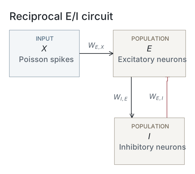
Parameters
Model values are read from original native snapshots through the selected presentation’s compute ancestry. Paired values are E / I. Initializer parent means and SDs describe the original weight distributions, in µS for conductance projections and dimensionless for the current-based readout; they are not measured trained-weight statistics. Missing snapshots or fields are unavailable; current recipes and historical copied tables are not substituted. The recorded configuration identifies the input, numerical and analysis choices of that computation; it does not establish a separate upstream training protocol.
| Parameter | Private input | Shared input |
|---|---|---|
| Network | ||
| E / I neurons | Unavailable / Unavailable | Unavailable / Unavailable |
| Output neurons | Unavailable | Unavailable |
| Neurons | ||
| Capacitance, E / I (nF) | Unavailable / Unavailable | Unavailable / Unavailable |
| Leak conductance, E / I (µS) | Unavailable / Unavailable | Unavailable / Unavailable |
| Resting voltage, E / I (mV) | Unavailable / Unavailable | Unavailable / Unavailable |
| Threshold, E / I (mV) | Unavailable / Unavailable | Unavailable / Unavailable |
| Reset, E / I (mV) | Unavailable / Unavailable | Unavailable / Unavailable |
| Refractory period, E / I | Unavailable / Unavailable | Unavailable / Unavailable |
| Synapses and weights | ||
| Input→E synapse | Unavailable / Unavailable | Unavailable / Unavailable |
| E→I synapse | Unavailable / Unavailable | Unavailable / Unavailable |
| I→E synapse | Unavailable / Unavailable | Unavailable / Unavailable |
| E→Output synapse | Unavailable / Unavailable | Unavailable / Unavailable |
| Input→E initializer parent mean / SD | Unavailable / Unavailable | Unavailable / Unavailable |
| E→I initializer parent mean / SD | Unavailable / Unavailable | Unavailable / Unavailable |
| I→E initializer parent mean / SD | Unavailable / Unavailable | Unavailable / Unavailable |
| E→Output initializer parent mean / SD | Unavailable / Unavailable | Unavailable / Unavailable |
| Native parameter stage | Unavailable | Unavailable |
| Input and simulation | ||
| Timestep (ms) | Unavailable | Unavailable |
| Duration (ms) | 1000 | 1000 |
| Evaluation samples | Unavailable | Unavailable |
| Seeds | 42 | 42 |
| Input rate (Hz) | 100 | 100 |
| Post-burn exclusion (ms) | 100 | 100 |
| Readout and training | ||
| Output neuron model | Unavailable | Unavailable |
| Epochs | Unavailable | Unavailable |
| Checkpoint role | Unavailable | Unavailable |
| Checkpoint purpose | Unavailable | Unavailable |
| Analysis | ||
| Frequency search (Hz) | Unavailable | Unavailable |
| Count-bin width (ms) | 1 | 1 |
| Autocorrelation maximum lag (ms) | 100 | 100 |
Dataset
Upstream: —
Downstream: exp110 — Manuscript
Current runset
| Run | Date | Duration | Size | Evidence | Storage | Ran on | Verification |
|---|---|---|---|---|---|---|---|
| exp054-r017-present | 3s | 783.2 KB | Current | R2 | Local | Local: absent; R2: catalog-verified | |
| exp054-r016-analyse | 4s | 711.2 KB | Current | R2 | Local | Local: absent; R2: catalog-verified | |
| exp054-r015-compute | 7m 37s | 11.3 MB | Current | R2 | Local | Local: absent; R2: catalog-verified |