Switching On the Inhibitory Loop
Enabling an inhibitory loop after feedforward training reduced excitatory firing but lowered classification accuracy; the experiment does not isolate a benefit of gamma timing.
Abstract
We asked what happens when reciprocal inhibition is enabled after feedforward training. We held the learned input and readout weights fixed and varied bidirectional E↔I coupling in three MNIST classifiers. At full loop strength, mean E rate fell from 86 to 7 Hz, while test accuracy fell by 47 percentage points. This demonstrates post-training rate suppression under these conditions, without isolating a benefit of gamma timing or testing whether retraining could recover accuracy.
Results
Loop-strength rates and accuracy
At full loop strength, E rate fell from approximately 86 to 7 Hz, I rate reached 40 Hz, and accuracy fell by 47 percentage points. Because both coupling directions varied, lower activity alone does not identify a causal benefit of rhythm (Fig. 1).

Figure 1: Reanalysed inference observations; no retraining. (A) Seed-42 raster with the loop off and (B) with the loop fully enabled, for the same digit-7 test image each shows 200 E neurons (black) and 64 I neurons (red). (C) Population rates and (D) accuracy on 1000 test images per seed; curves show means ± sample SD across seeds 42–44.
Loop-strength PING rasters
Burst grouping increased across the sampled loop strengths. These illustrative panels do not estimate gamma frequency or establish a continuous transition (Fig. 2).

Figure 2: Seed 42, the same digit-7 test image, at bidirectional loop strengths (A–F) , respectively. Learned input and readout weights were fixed; recurrent E↔I weights were initialized at each strength without training. Rows show the same sampled 200 E and 64 I neurons over 200 ms.
Methods
We reused networks from the exp022 — MNIST and reanalysed recorded inference observations. No new training or simulation was performed for this account.
-
Reuse trained classifiers. MNIST handwritten digits [1] supplied 6,300 training and 700 validation images from the official training partition. Conductance-based leaky-integrate-and-fire networks had 784 Poisson input channels, 1,024 excitatory (E), 256 inhibitory (I), and 10 output neurons; pixels set rates up to 25 Hz. Input and readout weights trained for 50 epochs; class scores were mean pre-reset output voltages. We selected the minimum mean validation cross-entropy over three fixed encoding draws, breaking ties by accuracy and then earliest epoch, rather than using final-epoch weights.
-
Enable the loop after training. Three feedforward controls, seeds 42–44, had no activity penalty or recurrent coupling during training. Dimensionless strength took eleven values from 0 to 1 in steps of 0.1; it set E→I and I→E initializer means to and , respectively, with standard deviations one tenth of those means and normalization by source population size. These lower-clamped normal weights replaced the zero recurrent matrices; learned input and readout weights stayed fixed, and E→E and I→I coupling stayed zero. The same network seed was reused across strengths; no optimization followed the intervention.
-
Evaluate responses. Each strength used the same 1000 images from the official 10000-image test partition, with 200 ms presentations and 0.1 ms steps. Accuracy counted correct classifications; rates included all neurons and all evaluated presentations:
Here denotes E or I, its neuron count, the number of presentations, their duration in seconds, and neuron ’s spike count during presentation ; is in hertz. Curves show means and sample standard deviations across the three networks; single-image rasters are illustrative.
-
Probe input drive. Auxiliary probes reused seed-42 classifiers trained with and without the loop. Uniform independent Poisson inputs covered 26 rates between 0 and 100 Hz, with 32 trials per rate; a separate trained-loop probe used one test image at ten maximum pixel rates from 0 to approximately 23.08 Hz. These recorded firing curves complement the exp023 — Turning the PING Loop On they are not additional loop-transfer accuracy evaluations.
Appendix: Training and probe settings
Training and probe settings are listed in Parameters.
The broader activity frontier contains 36 classifiers: two network configurations, three seeds, and six activity conditions (penalty off or ceilings of 25, 10, 5, 2.5 and 1 Hz). Its summaries preserve selected and final-epoch validation accuracy, final-epoch training E rate, and across-seed means and SEM; these are distinct from the inference measurements above. The loop-transfer comparison used only the three unpenalised feedforward classifiers. The exp025 — Inhibition, Accuracy and Firing describes the broader training design.
Feedforward and loop-enabled training used voltage-gradient damping of 1 and 1,000 respectively; this difference affects the auxiliary between-model comparisons, not the within-classifier inference intervention. Dale’s law was enforced, adaptive thresholds were disabled, and membrane time constants were not trained.
Illustrative snapshots use test-image index 0, not selection by digit class. A fixed pseudorandom sample selects 200 E and 64 I neurons for display; reported firing rates use the full populations. Uniform-input E+I overlays add the two population means without weighting by neuron count, and are not a whole-network mean. Neither the transfer rasters nor these firing curves provide a spectral gamma-frequency estimate. The accuracy decline is consistent with changing the trained network’s dynamics, but does not identify the readout as its sole cause or test recovery by retraining.
Network diagrams
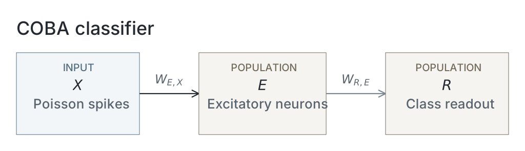
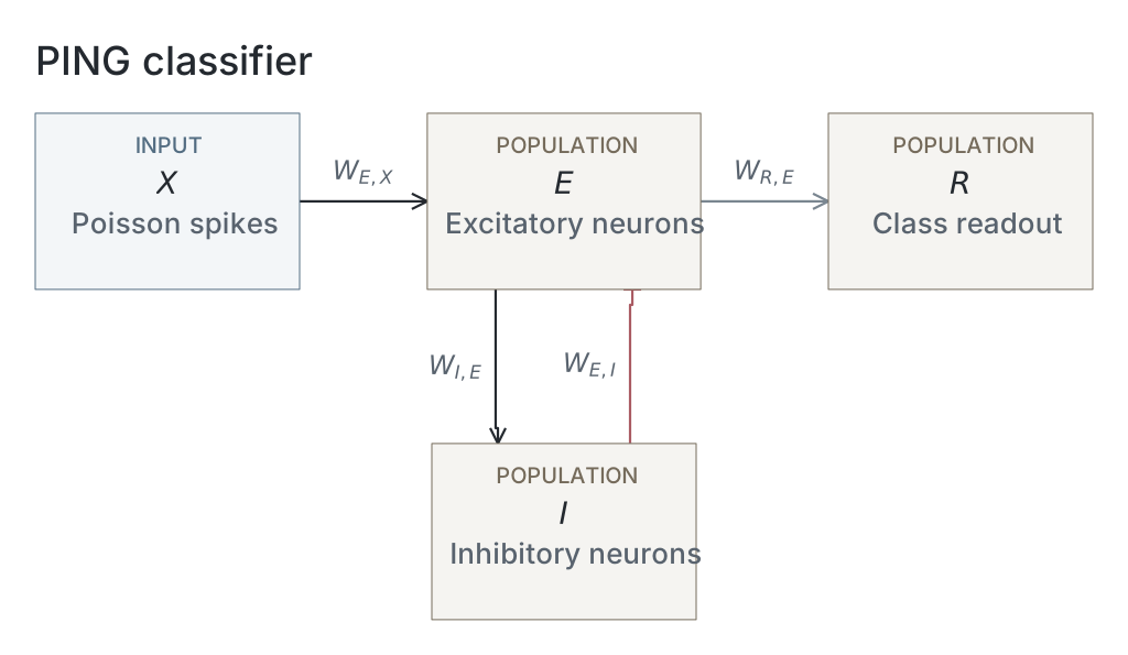
Parameters
Model values are read from original native snapshots through the selected presentation’s compute ancestry. Paired values are E / I. Initializer parent means and SDs describe the original weight distributions, in µS for conductance projections and dimensionless for the current-based readout; they are not measured trained-weight statistics. Missing snapshots or fields are unavailable; current recipes and historical copied tables are not substituted. The recorded configuration identifies the input, numerical and analysis choices of that computation; it does not establish a separate upstream training protocol.
| Parameter | Loop off | Loop on |
|---|---|---|
| Network | ||
| E / I neurons | Unavailable / Unavailable | Unavailable / Unavailable |
| Output neurons | Unavailable | Unavailable |
| Neurons | ||
| Capacitance, E / I (nF) | Unavailable / Unavailable | Unavailable / Unavailable |
| Leak conductance, E / I (µS) | Unavailable / Unavailable | Unavailable / Unavailable |
| Resting voltage, E / I (mV) | Unavailable / Unavailable | Unavailable / Unavailable |
| Threshold, E / I (mV) | Unavailable / Unavailable | Unavailable / Unavailable |
| Reset, E / I (mV) | Unavailable / Unavailable | Unavailable / Unavailable |
| Refractory period, E / I | Unavailable / Unavailable | Unavailable / Unavailable |
| Synapses and weights | ||
| Input→E synapse | Unavailable / Unavailable | Unavailable / Unavailable |
| E→I synapse | Unavailable / Unavailable | Unavailable / Unavailable |
| I→E synapse | Unavailable / Unavailable | Unavailable / Unavailable |
| E→Output synapse | Unavailable / Unavailable | Unavailable / Unavailable |
| Input→E initializer parent mean / SD | Unavailable / Unavailable | Unavailable / Unavailable |
| E→I initializer parent mean / SD | Unavailable / Unavailable | Unavailable / Unavailable |
| I→E initializer parent mean / SD | Unavailable / Unavailable | Unavailable / Unavailable |
| E→Output initializer parent mean / SD | Unavailable / Unavailable | Unavailable / Unavailable |
| Native parameter stage | Unavailable | Unavailable |
| Input and simulation | ||
| Timestep (ms) | Unavailable | Unavailable |
| Duration (ms) | Unavailable | Unavailable |
| Evaluation samples | Unavailable | Unavailable |
| Seeds | Unavailable | Unavailable |
| Input rate (Hz) | Unavailable | Unavailable |
| Post-burn exclusion (ms) | Unavailable | Unavailable |
| Readout and training | ||
| Output neuron model | Unavailable | Unavailable |
| Epochs | Unavailable | Unavailable |
| Checkpoint role | Unavailable | Unavailable |
| Checkpoint purpose | Unavailable | Unavailable |
| Analysis | ||
| Frequency search (Hz) | Unavailable | Unavailable |
| Count-bin width (ms) | Unavailable | Unavailable |
| Autocorrelation maximum lag (ms) | Unavailable | Unavailable |
Dataset
Downstream: exp110 — Manuscript
Current runset
| Run | Date | Duration | Size | Evidence | Storage | Ran on | Verification |
|---|---|---|---|---|---|---|---|
| exp038-r011-present | 21s | 683.2 KB | Current | R2 | HPC | Local: absent; R2: catalog-verified | |
| exp038-r010-analyse | 21s | 126.2 KB | Current | R2 | HPC | Local: absent; R2: catalog-verified | |
| exp038-r009-compute | 40m 35s | 996.5 KB | Current | R2 | HPC | Local: absent; R2: catalog-verified | |
| exp022-r015-compute | 12h 58m 52s | 3.6 GB | Current | R2 | HPC | Local: absent; R2: catalog-verified | |
| exp022-r007-compute | 11h 16m 8s | 3.6 GB | Current | R2 | HPC | Local: absent; R2: catalog-verified | |
| exp022-r001-compute | 2d 7h 4m 16s | 2 GB | Current | R2 | HPC | Local: absent; R2: catalog-verified |
References
- Y. LeCun, L. Bottou, Y. Bengio, and P. Haffner. “Gradient-based learning applied to document recognition.” Proceedings of the IEEE 86(11), 2278–2324 (1998). doi:10.1109/5.726791